Excel VLOOKUP Function
Summary
VLOOKUP is an Excel function to lookup and retrieve data from a specific column in table. VLOOKUP supports approximate and exact matching, and wildcards (* ?) for partial matches. The "V" stands for "vertical". Lookup values must appear in the first column of the table, with lookup columns to the right.
Purpose
Lookup a value in a table by matching on the first column
Return value
The matched value from a table.
Syntax
=VLOOKUP (value, table, col_index, [range_lookup])
Arguments
- value - The value to look for in the first column of a table.
- table - The table from which to retrieve a value.
- col_index - The column in the table from which to retrieve a value.
- range_lookup - [optional] TRUE = approximate match (default). FALSE = exact match.
Usage notes
VLOOKUP is designed to retrieve data in a table organized into vertical rows, where each row represents a new record. The "V" in VLOOKUP stands for vertical:
If you have data organized horizontally, use the HLOOKUP function.
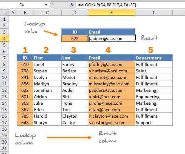
VLOOKUP only looks right
VLOOKUP requires a lookup table with lookup values in the left-most column. The data you want to retrieve (result values) can appear in any column to the right:
VLOOKUP retrieves data based on column number
When you use VLOOKUP, imagine that every column in the table is numbered, starting from the left. To get a value from a particular column, simply supply the appropriate number as the "column index":
=VLOOKUP(H3,B4:E13,2,FALSE) // first=VLOOKUP(H3,B4:E13,3,FALSE) // last=VLOOKUP(H3,B4:E13,4,FALSE) // email
VLOOKUP has two matching modes, exact and approximate
VLOOKUP has two modes of matching: exact and approximate, which are controlled by the 4th argument, called "range_lookup". Set range_lookup to FALSE to force exact matching, and TRUE for approximate matching.
Important: range_lookup defaults to TRUE, so VLOOKUP will use approximate matching by default:
=VLOOKUP(value, table, column) // default, approximate match=VLOOKUP(value, table, column, TRUE) // approximate match=VLOOKUP(value, table, column, FALSE) // exact match
Example 1: Exact match
In most cases, you'll probably want to use VLOOKUP in exact match mode. This makes sense when you have a unique key to use as a lookup value, for example, the movie title in this data:
The formula in H6 to lookup year based on an exact match of movie title is:
=VLOOKUP(H4,B5:E9,2,FALSE) // FALSE = exact match
Example 2: Approximate match
You'll want to use approximate mode in cases when you're looking for the best match, not an exact match. A classic example is finding the right commission rate based on a monthly sales number. In this case, you want VLOOKUP to get you the best match for a given lookup value. In the example below, the formula in D5 performs an approximate match to retrieve the correct commission.
=VLOOKUP(C5,$G$5:$H$10,2,TRUE) // TRUE = approximate match
Note: your data must be sorted in ascending order by lookup value when you use approximate match mode with VLOOKUP.
More about VLOOKUP
Other notes
- Range_lookup controls whether value needs to match exactly or not. The default is TRUE = allow non-exact match.
- Set range_lookup to FALSE to require an exact match and TRUE to allow a non-exact match.
- If range_lookup is TRUE (the default setting), a non-exact match will cause the VLOOKUP function to match the nearest value in the table that is still less than value.
- When range_lookup is omitted, the VLOOKUP function will allow a non-exact match, but it will use an exact match if one exists.
- If range_lookup is TRUE (the default setting) make sure that lookup values in the first row of the table are sorted in ascending order. Otherwise, VLOOKUP may return an incorrect or unexpected value.
- If range_lookup is FALSE (require exact match), values in the first column of table do not need to be sorted.