Highlight cells that contain one of many

Generic formula

=SUMPRODUCT(--ISNUMBER(SEARCH(things,A1)))>0

Related formulas

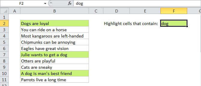
Highlight cells that contain

Explanation

To highlight cells that contain one of many text strings, you can use a formula based on the functions ISNUMBER and SEARCH, together with the SUMPRODUCT function.

In the example shown, the conditional formatting applied to B4:B11 uses this formula:

=SUMPRODUCT(--ISNUMBER(SEARCH(things,B4)))>0

How this formula works

Working from the inside out, this part of the formula searches each cell in B4:B11 for all values in the named range "things":

--ISNUMBER(SEARCH(things,B4)

The SEARCH function returns the position of the value if found, and and the #VALUE error if not found. For B4, the results come back in an array like this:

{8;#VALUE!;#VALUE!}

The ISNUMBER function changes all results to TRUE or FALSE:

{TRUE;FALSE;FALSE}

The double negative in front of ISNUMBER forces TRUE/FALSE to 1/0:

{1;0;0}

The SUMPRODUCT function then adds up the results, which is tested against zero:

=SUMPRODUCT({1;0;0})>0

Any non-zero result means at least one value was found, so the formula returns TRUE, triggering the rule.

Case-sensitive option

SEARCH is not case-sensitive. If you need to check case as well, just replace SEARCH with FIND like so:

=SUMPRODUCT(--ISNUMBER(FIND(things,A1)))>0