Cell contains one of many with exclusions
Generic formula
=(SUMPRODUCT(--ISNUMBER(SEARCH(include,A1)))>0)*(SUMPRODUCT(--ISNUMBER(SEARCH(exclude,A1)))=0)
Related formulas
Cell contains one of many things
Cell contains all of many things
Get first match cell contains
Cell contains specific text
Value exists in a range
Cell contains which things
If cell contains one of many things
Explanation
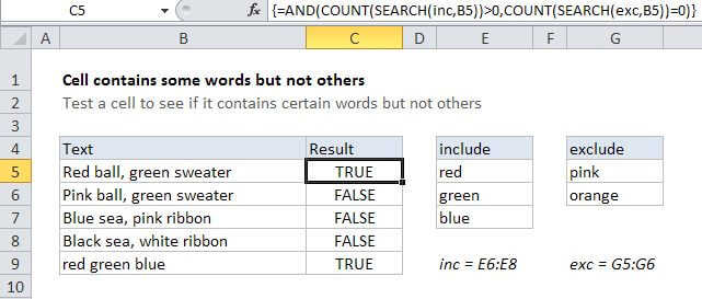
To test a cell for one of many strings, while excluding others, you can use a formula based on the SEARCH, ISNUMBER, and SUMPRODUCT functions.
In the example shown the formula in C5 is:
=(SUMPRODUCT(--ISNUMBER(SEARCH(include,B5)))>0)*(SUMPRODUCT(--ISNUMBER(SEARCH(exclude,B5)))=0)
where "include" is the named range E5:E9, and "exclude" is the named range G5:G6.
How this formula works
At the core, this formula uses the SEARCH function to look for multiple strings inside a cell. Inside the left SUMPRODUCT, SEARCH looks for all strings in the named range "include".
In the right SUMPRODUCT, SEARCH looks for all strings in the named range "exclude".
In both parts of the formula, SEARCH returns numeric positions when strings are found, and errors when not. The ISNUMBER functions converts the numbers to TRUE and errors to FALSE, and the double negative converts the TRUE FALSE values to 1 and 0.
The result at this point looks like this:
=(SUMPRODUCT({1;0;0;0;0})>0)*(SUMPRODUCT({0;0})=0)
Then:
=(1>0)*(0=0)=TRUE*FALSE=1
Note: this formula returns either 1 or zero, which are handled like TRUE and FALSE in formulas, conditional formatting, or data validation.