Hyperlink to first blank cell
Generic formula
=HYPERLINK("#"&CELL("address",INDEX(range,MATCH(bignum,range)+1)),"First blank")Related formulas
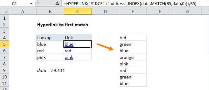
Hyperlink to first match
Build hyperlink with VLOOKUP
Last row in numeric data
Last row in text data
Last row in mixed data with blanks
Explanation
To create hyperlinks to the first match in a lookup, you can use a formula based on the HYPERLINK function, with help from CELL, INDEX and MATCH.
In the example shown, the formula in C5 is:
=HYPERLINK("#"&CELL("address",INDEX(C5:C100,MATCH(9.99E+307,C5:C100)+1)),"First blank")
This formula generates a working hyperlink to the first blank cell in column C.
How this formula works
Working from the inside out, we use MATCH to locate the relative position of the last entry in column C:
MATCH(9.99E+307,C5:C100)
Basically, we are giving match a "big number" it will never find in approximate match mode. In this mode match will "step back" the last numeric value. This works in this case because all values in C are numeric, and there are no blanks. For other situations, see other "last row" formulas linked on this page.
Next, we use INDEX to get the address of the "entry after the last entry" like this:
INDEX(C5:C100,6))
For array, we give INDEX C:C100 which represents the range we care about. For row number, we give INDEX the result returned by MATCH + 1. In this example, this simplifies to:
INDEX(C5:C100,6)
This appears to return the value at C10 but in fact INDEX actually returns an address ($C$10), which we extract with the CELL function and concatenate to the "#" character:
=HYPERLINK("#"&CELL($C$10)
In this end, this is what goes into the HYPERLINK function:
=HYPERLINK("#$C$10","First blank")
The HYPERLINK function then constructs a clickable link to cell C10 on the same sheet, with "First link" as the link text.