Sum if cell contains text in another cell
Generic formula
=SUMIF(range,"*"&A1&"*",sum_range)
Related formulas
Sum if cells contain specific text
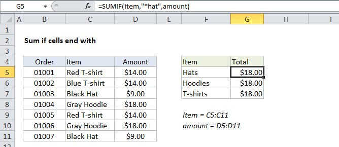
Sum if begins with
Sum if not blank
Sum if cells are equal to
Sum if cells are not equal to
Sum if equal to either x or y
Explanation
To sum if cells contain specific text in another cell, you can use the SUMIF function with a wildcard and concatenation.
In the example shown, cell G6 contains this formula:
=SUMIF(C5:C11,"*"&F6&"*",D5:D11)
This formula sums the amounts in column D when a value in column C contains the text in cell F6.
How the formula works
The SUMIF function supports wildcards. An asterisk (*) means "one or more characters", while a question mark (?) means "any one character".
These wildcards allow you to create criteria such as "begins with", "ends with", "contains 3 characters" and so on.
So, for example, you use criteria like "*hat*" to match text anywhere in a cell.
In this case, we want to match the text in F6. We can't write the criteria like "*F6*" because that will match only the literal text "F6".
Instead, we need to use the concatenation operator (&) to join a reference to F6 to asterisks (*):
"*"&F6&"*"
When Excel evaluates this argument inside the SUMIF function, it will "see" this: "*Hoodie*".
Note that SUMIF is not case-sensitive.
Alternative with SUMIFS
You can also use the SUMIFS function. SUMIFS can handle multiple criteria, and the order of the arguments is different from SUMIF. The equivalent SUMIFS formula is:
=SUMIFS(D5:D11,C5:C11,"*"&F6&"*")
Notice that the sum range always comes first in the SUMIFS function.